This notebook contains an excerpt from the Python Programming and Numerical Methods - A Guide for Engineers and Scientists, the content is also available at Berkeley Python Numerical Methods.
The copyright of the book belongs to Elsevier. We also have this interactive book online for a better learning experience. The code is released under the MIT license. If you find this content useful, please consider supporting the work on Elsevier or Amazon!
< 24.4 FFT in Python | Contents | CHAPTER 25. Introduction to Machine Learning >
Summary
We learned the basics of the waves, frequency, period, amplitude and wavelength are the characteristics of the waves.
The Discrete Fourier Transform (DFT) is a way to transform a signal from time domain to frequency domain using the sum of a sequence of sine waves.
The Fast Fourier Transform (FFT) is an algorithm to calculate the DFTs efficiently by taking advantage of the symmetry properties in DFT.
Problems
A task assigned to you to measure the temperature of the room. Thus everyday at noon, you measure the temperature and record the value. You measured for 30 days. What’s the frequency of the temperature signal you get?
What’s the relationship of the frequency and period of a wave?
What’s the difference of period and wavelength? What are the similarities between them?
What are the time domain and frequency domain representation of a signal?
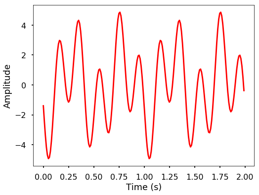
Generate two signals, signal 1 is a sine wave with 5 Hz, amplitude 3 and phase shift 3, signal 2 is a sine wave with 2 Hz, amplitude 2 and phase shift -2. Plot the signal for 2 seconds. Test Cases:
# sampling rate
sr = 100
# sampling interval
ts = 1.0/sr
t = np.arange(0,2,ts)

freq = 5.
x = 3*np.sin(2*np.pi*freq*t + 3)

freq = 2
x += 2*np.sin(2*np.pi*freq*t - 2)


plt.figure(figsize = (8, 6))
plt.plot(t, x, 'r')
plt.ylabel('Amplitude')
plt.xlabel('Time (s)')
plt.show()

Sample the signal you generated in problem 5 using a sampling rate 5, 10, 20, 50, and 100 Hz, and see the differences between different sampling rates.
Given a signal t = [0, 1, 2, 3], and y = [0, 3, 2, 0], find the real DFT of X. Write the expression for the inverse DFT. Note that, don’t use Python to find the results, instead write out the equations and calculate the values.
What are the amplitude and phase of the DFT values for a signal?
We implement the DFT previously, can you implement the inverse Discrete Fourier Transform in Python similarly?
Use the DFT function and inverse DFT we implemented and generate the amplitude spectrum for the signal you generated in problem 5. Normalize the DFT amplitude to get the correct corresponding time domain amplitude.
Can you describe the tricks used in FFT to make the computation faster?
Use the fft and ifft function from scipy to repeat problem 10.
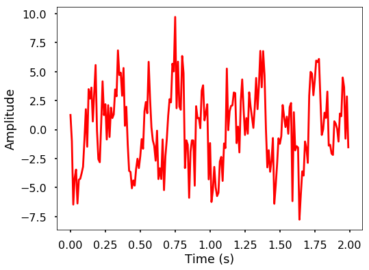
Adding a random normal distribution noise into the signal in problem 5 using numpy and plot the FFT amplitude spectrum, what do you see? The signal with noise will be shown as the following test case.
Test Case:
np.random.seed(10)
x_noise = x + \
  np.random.normal(0, 2, size = len(x))

plt.figure(figsize = (8, 6))
plt.plot(t, x_noise, 'r')
plt.ylabel('Amplitude')
plt.xlabel('Time (s)')
plt.show()

< 24.4 FFT in Python | Contents | CHAPTER 25. Introduction to Machine Learning >
