Least Squares Regression in Python¶

Recall that if we enumerate the estimation of the data at each data point, $x_i$, this gives us the following system of equations:

\[\begin{eqnarray*} &&\hat{y}(x_1) = {\alpha}_1 f_1(x_1) + {\alpha}_2 f_2(x_1) + \cdots + {\alpha}_n f_n(x_1),\\ &&\hat{y}(x_2) = {\alpha}_1 f_1(x_2) + {\alpha}_2 f_2(x_2) + \cdots + {\alpha}_n f_n(x_2),\\ &&\qquad\qquad\qquad\qquad\qquad \cdots\\ &&\hat{y}(x_m) = {\alpha}_1 f_1(x_m) + {\alpha}_2 f_2(x_m) + \cdots + {\alpha}_n f_n(x_m). \end{eqnarray*}\]

If the data was absolutely perfect (i.e., no noise), then the estimation function would go through all the data points, resulting in the following system of equations:

\[\begin{eqnarray*} &&y_1 = {\alpha}_1 f_1(x_1) + {\alpha}_2 f_2(x_1) + \cdots + {\alpha}_n f_n(x_1),\\ &&y_2 = {\alpha}_1 f_1(x_2) + {\alpha}_2 f_2(x_2) + \cdots + {\alpha}_n f_n(x_2),\\ &&\qquad\qquad\qquad\qquad\cdots\\ &&y_m = {\alpha}_1 f_1(x_m) + {\alpha}_2 f_2(x_m) + \cdots + {\alpha}_n f_n(x_m). \end{eqnarray*}\]

If we take $A$ to be as defined previously, this would result in the matrix equation $$ Y = A{\beta}. $$

However, since the data is not perfect, there will not be an estimation function that can go through all the data points, and this system will have $\textit{no solution}$. Therefore, we need to use the least square regression that we derived in the previous two sections to get a solution.

\[{\beta} = (A^T A)^{-1} A^T Y\]

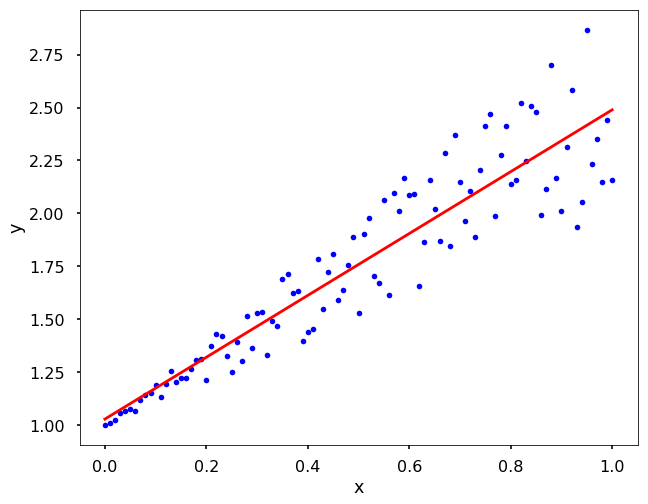
TRY IT! Consider the artificial data created by $\textit{x = np.linspace(0, 1, 101)}$ and $\textit{y = 1 + x + x * np.random.random(len(x))}$. Do a least squares regression with an estimation function defined by $\hat{y}=\alpha_1x+\alpha_2$. Plot the data points along with the least squares regression. Note that we expect $\alpha_1=1.5$ and $\alpha_2=1.0$ based on this data. Due to the random noise we added into the data, your results maybe slightly different.

Use direct inverse method¶

import numpy as np
from scipy import optimize
import matplotlib.pyplot as plt

plt.style.use('seaborn-poster')

# generate x and y
x = np.linspace(0, 1, 101)
y = 1 + x + x * np.random.random(len(x))

# assemble matrix A
A = np.vstack([x, np.ones(len(x))]).T

# turn y into a column vector
y = y[:, np.newaxis]

# Direct least square regression
alpha = np.dot((np.dot(np.linalg.inv(np.dot(A.T,A)),A.T)),y)
print(alpha)

[[1.459573  ]
 [1.02952189]]

# plot the results
plt.figure(figsize = (10,8))
plt.plot(x, y, 'b.')
plt.plot(x, alpha[0]*x + alpha[1], 'r')
plt.xlabel('x')
plt.ylabel('y')
plt.show()

../_images/chapter16.04-Least-Squares-Regression-in-Python_8_0.png

In Python, there are many different ways to conduct the least square regression. For example, we can use packages as numpy, scipy, statsmodels, sklearn and so on to get a least square solution. Here we will use the above example and introduce you more ways to do it. Feel free to choose one you like.

Use the pseudoinverse¶

We talked before that the $(A^T A)^{-1} A^T$ is called the pseudo-inverse, therefore, we could use the pinv function in numpy to directly calculate it.

pinv = np.linalg.pinv(A)
alpha = pinv.dot(y)
print(alpha)

[[1.459573  ]
 [1.02952189]]

Use numpy.linalg.lstsq¶

Actually, numpy has already implemented the least square methods that we can just call the function to get a solution. The function will return more things than the solution itself, please check the documentation for details.

alpha = np.linalg.lstsq(A, y, rcond=None)[0]
print(alpha)

[[1.459573  ]
 [1.02952189]]

Use optimize.curve_fit from scipy¶

This scipy function is actually very powerful, that it can fit not only linear functions, but many different function forms, such as non-linear function. Here we will show the linear example from above. Note that, using this function, we don’t need to turn y into a column vector.

# generate x and y
x = np.linspace(0, 1, 101)
y = 1 + x + x * np.random.random(len(x))

def func(x, a, b):
    y = a*x + b
    return y

alpha = optimize.curve_fit(func, xdata = x, ydata = y)[0]
print(alpha)

[1.44331612 1.0396133 ]

< 16.3 Least Squares Regression Derivation (Multivariable Calculus) | Contents | 16.5 Least Square Regression for Nonlinear Functions >

Python Numerical Methods

Least Squares Regression in Python¶

Use direct inverse method¶

Use the pseudoinverse¶

Use numpy.linalg.lstsq¶

Use optimize.curve_fit from scipy¶