

This notebook contains an excerpt from the Python Programming and Numerical Methods - A Guide for Engineers and Scientists, the content is also available at Berkeley Python Numerical Methods.
The copyright of the book belongs to Elsevier. We also have this interactive book online for a better learning experience. The code is released under the MIT license. If you find this content useful, please consider supporting the work on Elsevier or Amazon!
< 17.5 Newton’s Polynomial Interpolation | Contents | CHAPTER 18. Series >
Summary
Given a set of reliable data points, interpolation is a method of estimating dependent variable values for independent variable values not in our data set.
Linear, Cubic Spline, Lagrange and Newton’s polynomial interpolation are common interpolating methods.
Problems
Write a function my_lin_interp(x, y, X), where x and y are arrays containing experimental data points, and X is an array. Assume that x and X are in ascending order and have unique elements. The output argument, Y, should be an array, the same size as X, where Y[i] is the linear interpolation of X[i]. You should not use interp from numpy or interp1d from scipy.
Write a function my_cubic_spline(x, y, X), where x and y are arrays containing experimental data points, and X is an array. Assume that x and X are in ascending order and have unique elements. The output argument, Y, should be an array, the same size as X, where Y[i] is cubic spline interpolation of X[i]. You may not use interp1d or CubicSpline.
Write a function my_nearest_neighbor(x, y, X), where x and y are arrays containing experimental data points, and X is an array. Assume that x and X are in ascending order and have unique elements. The output argument, Y, should be an array, the same size as X, where Y[i] is the nearest neighbor interpolation of X[i]. That is, Y[i] should be the y[j] where x[j] is the closest independent data point of X[i]. You may not use interp1d from scipy.
Think of a situation where using nearest neighbor interpolation would be superior to cubic spline interpolation.
Write a function my_cubic_spline_flat(x, y, X), where x and y are arrays containing experimental data points, and X is an array. Assume that x and X are in ascending order and have unique elements. The output argument, Y, should be an array, the same size as X, where Y[i] is the cubic spline interpolation of X[i]. However, instead of the constraints we introduced before, use \(S'_1(x_1)=0\) and \(S'_{n-1}(x_n)=0\).
Write a function my_quintic_spline(x, y, X), where x and y are arrays containing experimental data points, and X is an array. Assume that x and X are in ascending order and have unique elements. The output argument, Y, should be an array, the same size as X, where Y[i] is the quintic spline interpolation of X[i]. You will need to use additional endpoint constraints to come up with enough constraints. You may use endpoint constraints at your discretion.
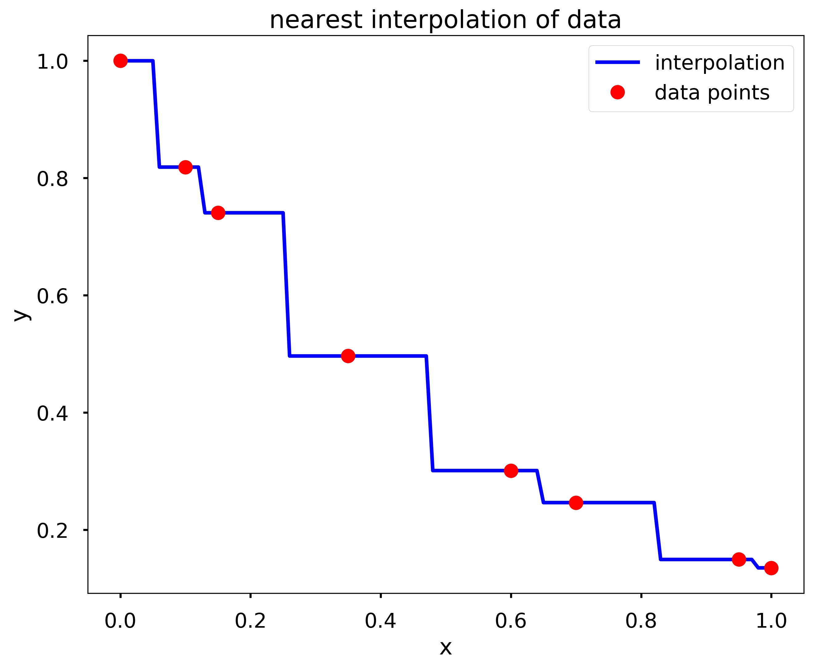
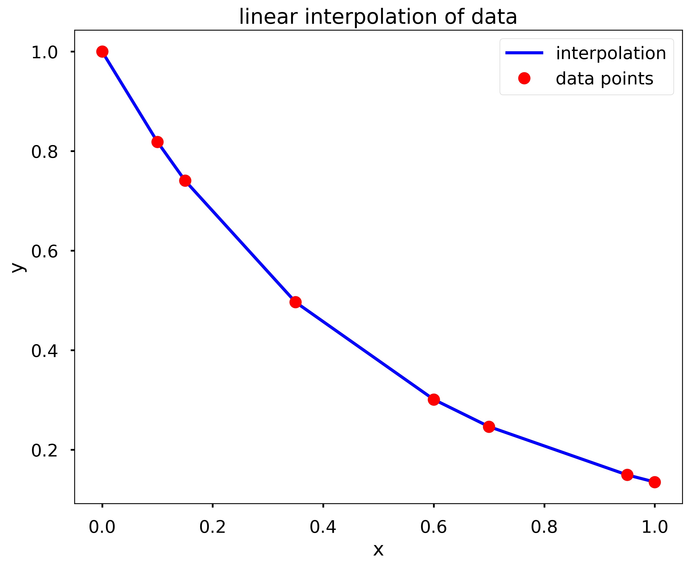
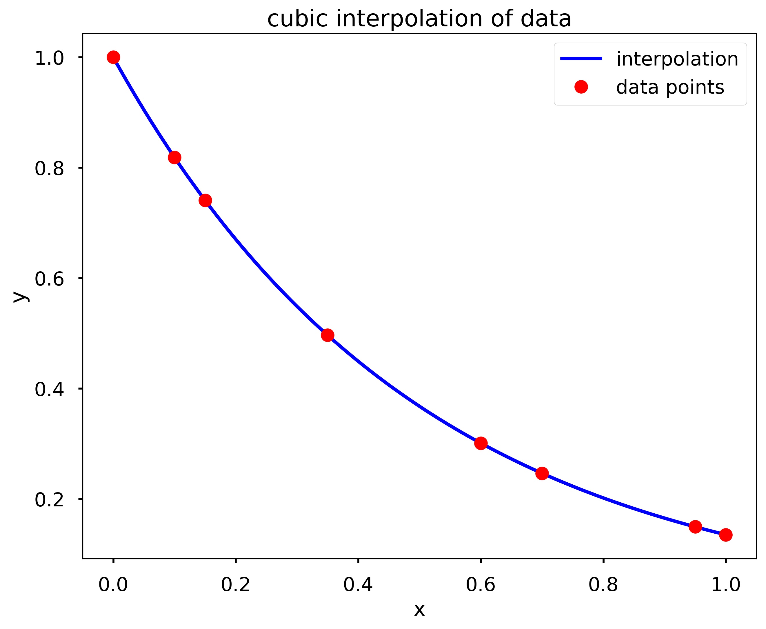
Write a function my_interp_plotter(x, y, X, option), where x and y are arrays containing experimental data points, and X is an array containing the coordinates for which an interpolation is desired. The input argument option should be a string, either ‘linear’, ‘spline’, or ‘nearest’. Your function should produce a plot of the data points \((x, y)\) marked as red circles. and the points \((X, Y)\), where X is the input and Y is the interpolation at the points contained in X defined by the input argument specified by option. The points \((X, Y)\) should be connected by a blue line. Be sure to include title, axis labels, and a legend. Hint: You should use interp1d from scipy, and checkout the kind option.
Test cases:
x = np.array([0, .1, .15, .35, .6, .7, .95, 1])
y = np.array([1, 0.8187, 0.7408, 0.4966, 0.3012, 0.2466, 0.1496, 0.1353])

my_interp_plotter(x, y, np.linspace(0, 1, 101), 'nearest')
my_interp_plotter(x, y, np.linspace(0, 1, 101), 'linear')
my_interp_plotter(x, y, np.linspace(0, 1, 101), 'cubic')
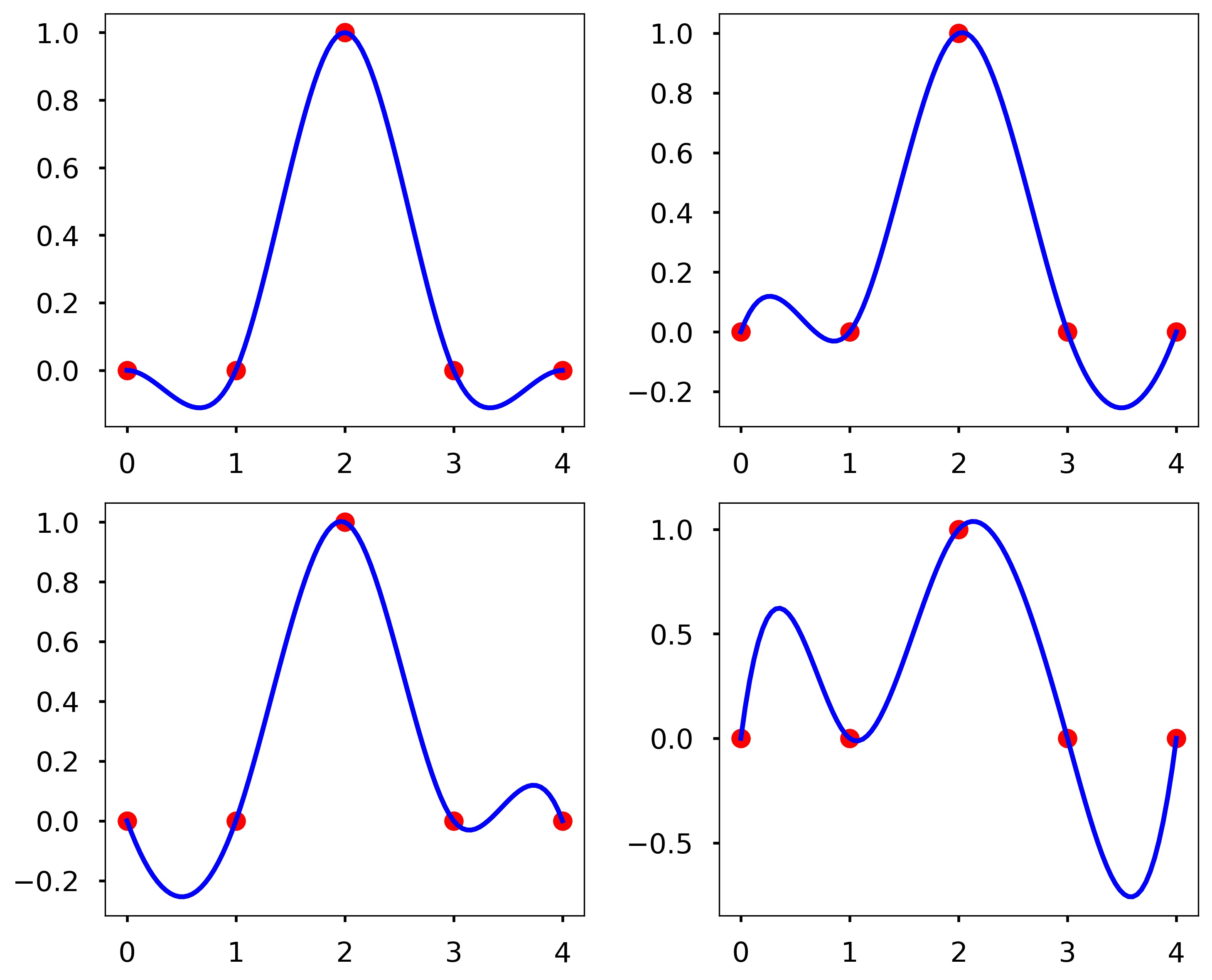
Write a function my_D_cubic_spline(x, y, X, D), where the output Y is the cubic spline interpolation at X taken from the data points contained in x and y. However, instead of the standard pinned endpoint conditions (i.e., \(S''_1(x_1) = 0\) and \(S''_{n-1}(x_n) = 0\)) you should use the endpoint conditions \(S^{\prime}_1(x_1) = D\) and \(S^{\prime}_{n-1}(x_n) = D\) (i.e., the slopes of the interpolating polynomials at the endpoints is \(D\)).
Test cases:
x = [0, 1, 2, 3, 4]
y = [0, 0, 1, 0, 0]
X = np.linspace(0, 4, 101)

# Solution: Y = 0.54017857
Y = my_D_cubic_spline(x, y, 1.5, 1)

plt.figure(figsize = (10, 8))
plt.subplot(221)
plt.plot(x, y, 'ro', X, my_D_cubic_spline(x, y, X, 0), 'b')
plt.subplot(222)
plt.plot(x, y, 'ro', X, my_D_cubic_spline(x, y, X, 1), 'b')
plt.subplot(223)
plt.plot(x, y, 'ro', X, my_D_cubic_spline(x, y, X, -1), 'b')
plt.subplot(224)
plt.plot(x, y, 'ro', X, my_D_cubic_spline(x, y, X, 4), 'b')
plt.tight_layout()
plt.show()
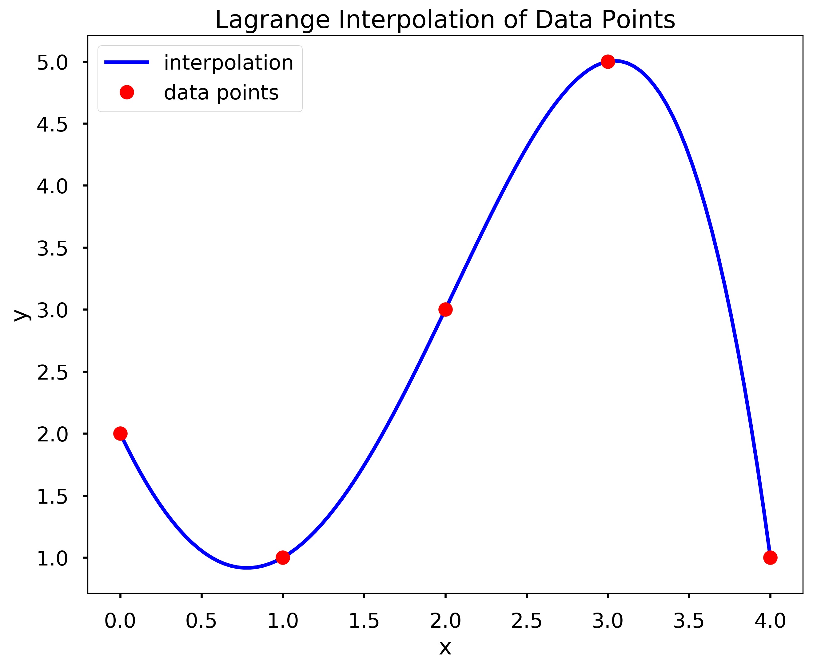
Write a function my_lagrange(x, y, X), where the output Y is the Lagrange interpolation of the data points contained in x and y computed at X. Hint: Use a nested for-loop, where the inner for-loop computes the product for the Lagrange basis polynomial and the outer loop computes the sum for the Lagrange polynomial. Don’t use the existing lagrange function from scipy.
Test cases
x = [0, 1, 2, 3, 4]
y = [2, 1, 3, 5, 1]

X = np.linspace(0, 4, 101)

plt.figure(figsize = (10,8 ))
plt.plot(X, my_lagrange(x, y, X), 'b', label = 'interpolation')
plt.plot(x, y, 'ro', label = 'data points')

plt.xlabel('x')
plt.ylabel('y')

plt.title(f'Lagrange Interpolation of Data Points')
plt.legend()
plt.show()
Fit the data x = [0, 1, 2, 3, 4], y = [2, 1, 3, 5, 1] using Newton’s polynomial interpolation.
< 17.5 Newton’s Polynomial Interpolation | Contents | CHAPTER 18. Series >