This notebook contains an excerpt from the Python Programming and Numerical Methods - A Guide for Engineers and Scientists, the content is also available at Berkeley Python Numerical Methods.
The copyright of the book belongs to Elsevier. We also have this interactive book online for a better learning experience. The code is released under the MIT license. If you find this content useful, please consider supporting the work on Elsevier or Amazon!
< 20.3 Approximating of Higher Order Derivatives | Contents | 20.5 Summary and Problems >
Numerical Differentiation with Noise
As stated earlier, sometimes \(f\) is given as a vector where \(f\) is the corresponding function value for independent data values in another vector \(x\), which is gridded. Sometimes data can be contaminated with noise, meaning its value is off by a small amount from what it would be if it were computed from a pure mathematical function. This can often occur in engineering due to inaccuracies in measurement devices or the data itself can be slightly modified by perturbations outside the system of interest. For example, you may be trying to listen to your friend talk in a crowded room. The signal \(f\) might be the intensity and tonal values in your friend’s speech. However, because the room is crowded, noise from other conversations are heard along with your friend’s speech, and he becomes difficult to understand.
To illustrate this point, we numerically compute the derivative of a simple cosine wave corrupted by a small sin wave. Consider the following two functions:
and
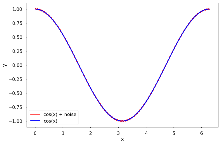
where \(0 < \epsilon\ll1\) is a very small number and \(\omega\) is a large number. When \(\epsilon\) is small, it is clear that \(f\simeq f_{\epsilon,\omega}\). To illustrate this point, we plot \(f_{\epsilon,\omega}(x)\) for \(\epsilon = 0.01\) and \(\omega = 100\), and we can see it is very close to \(f(x)\), as shown in the following figure.
import numpy as np
import matplotlib.pyplot as plt
plt.style.use('seaborn-poster')
%matplotlib inline
x = np.arange(0, 2*np.pi, 0.01)
# compute function
omega = 100
epsilon = 0.01

y = np.cos(x)
y_noise = y + epsilon*np.sin(omega*x)

# Plot solution
plt.figure(figsize = (12, 8))
plt.plot(x, y_noise, 'r-', \
         label = 'cos(x) + noise')
plt.plot(x, y, 'b-', \
         label = 'cos(x)')

plt.xlabel('x')
plt.ylabel('y')

plt.legend()
plt.show()

The derivatives of our two test functions are
and
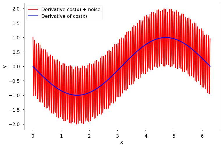
Since \(\epsilon\omega\) may not be small when \(\omega\) is large, the contribution of the noise to the derivative may not be small. As a result, the derivative (analytic and numerical) may not be usable. For instance, the following figure shows \(f^{\prime}(x)\) and \(f^{\prime}_{\epsilon,\omega}(x)\) for \(\epsilon = 0.01\) and \(\omega = 100\).
x = np.arange(0, 2*np.pi, 0.01)
# compute function
y = -np.sin(x)
y_noise = y + epsilon*omega*np.cos(omega*x)

# Plot solution
plt.figure(figsize = (12, 8))
plt.plot(x, y_noise, 'r-', \
         label = 'Derivative cos(x) + noise')
plt.plot(x, y, 'b-', \
         label = 'Derivative of cos(x)')

plt.xlabel('x')
plt.ylabel('y')

plt.legend()
plt.show()

< 20.3 Approximating of Higher Order Derivatives | Contents | 20.5 Summary and Problems >
